Viewing Activity
The "viewing activity" web interface is parsing json; no scraping needed!
The actual data returned incluces a lot of useful information too. Though it's not displayed, we have time-stamped view time, series title, and duration.
It appears as though duration is not view duration but the duration of the episode/movie. I think there is not a good way to see if something was only partially watched. This is inflating summary metrics.
pulling data
- https://www.netflix.com/WiViewingActivity
- inspect element -> network console
- ctrl + end (scroll to bottom to load)
right click -> copy as curl
- increment ?pg= and can discard rest of url
- only need memclid, SecureNetflixId, and NetflixId from Cookie
- increasing page size seems to have no effect, always 100 items returned
[ ! -d netflix ] && mkdir netflix
for i in {1..10}; do
    curl "https://www.netflix.com/api/shakti/adc049f7/viewingactivity?pg=$i" \
        -H 'Cookie: memclid=XXXX; SecureNetflixId=XXX; NetflixId=XXXX' \
        > netflix/$i.json
done
Reading in
R has some nice tools to read in the data.
jsonlitecreates a dataframe from a list of dicts automatically.lubridatemakes working with dates easy
  library(jsonlite)
  library(lubridate)
  library(dplyr)
  library(ggplot2)
  library(cowplot)

  flist <- Sys.glob('netflix/*json')
  dlist <- lapply(flist, function(f) { fromJSON(f)$viewedItems } )
  d <- Reduce(rbind,dlist)
  # date column is *1000 unix epoch ==  dateStr
  # see: as.POSIXct(d$date/1000,origin="1970-01-01")

  # get only this last year
  stopdate <- as.numeric(lubridate::now() - years(1)) * 1000
  d.year <-
      d %>%
      filter( date >= stopdate)  %>%
      mutate(datetime = with_tz(as_datetime(date/1000),'America/New_York'),
             dur.min = duration/60 ) %>%
      filter( dur.min > 1)  %>%
      arrange(-date)
Summarizing
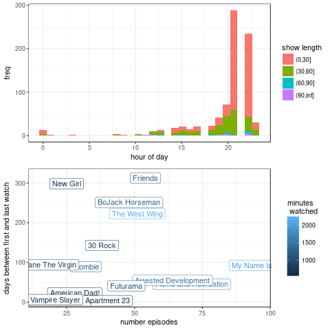
Plotting what hour of the day gets the most TV watching and what series are viewed the most.
  s <-
      d.year %>%
      group_by(seriesTitle) %>%
      summarise(total.min=sum(dur.min),
                n = n(),
                mindate = min(datetime),
                maxdate = max(datetime)) %>%
      mutate(span.days = as.numeric(maxdate-mindate)/(60*60*24),
             rank=rank(-n) ) %>%
      arrange(-n)

  p.topwatch <-
      s %>%
      filter(total.min > 500) %>%
      ggplot() +
      aes(x=n, y=span.days, color=total.min, label=seriesTitle) +
      #geom_point() +
      geom_label() +
      theme_bw() +
      labs(color="minutes\n watched",
           x="number episodes",
           y="days between first and last watch")

  p.hours <-
      ggplot(d.year) +
      aes(x = hour(datetime),
          fill = cut(dur.min, breaks=c(0,30,60,90,Inf))) +
      geom_histogram() +
      theme_bw() +
      labs(y='freq',
           x='hour of day',
           fill='show length')

  plot_grid(p.hours,p.topwatch,align='v',nrow=2)